Admixture Mapping

Admixture mapping tests whether local ancestry at a genomic region is associated with a phenotype in recently admixed individuals. Instead of asking whether a specific SNP allele is associated with a trait, we ask whether carrying ancestry from a source population at a local genomic window changes trait values after accounting for background ancestry and other covariates.

In this tutorial, we build a synthetic local ancestry dataset with a quantitative trait, run snputils.tools.run_admixture_mapping, and make a Manhattan plot from the resulting association table.

from pathlib import Path

import matplotlib.pyplot as plt
import numpy as np
import pandas as pd

from snputils.datasets import build_synthetic_admixture_dataset
from snputils.phenotype.genobj import CovariateObject, PhenotypeObject
from snputils.tools import run_admixture_mapping
from snputils.visualization import manhattan_plot, qq_plot

What the input represents

A local ancestry inference method usually produces one ancestry label per haplotype per genomic window. For a diploid sample, each window therefore has two ancestry labels: one for each haplotype. snputils stores that information in a LocalAncestryObject.

For each ancestry and each window, admixture mapping converts those two haplotype labels into an ancestry dosage: 0, 1, or 2 copies of the requested ancestry. The association model then tests whether that dosage is related to the phenotype.

Build a synthetic dataset

The synthetic trait below has a few sparse local ancestry effects plus global ancestry-like covariates, so the strongest signals should appear near the simulated causal windows while most tests remain null.

build_synthetic_admixture_dataset lives in snputils.datasets, and returns:

• laiobj: local ancestry calls for each haplotype and window.

• phenotype: a continuous trait generated from a few local ancestry effects, covariates, and noise.

• covar_matrix: covariates that include genome-wide ancestry-like summaries.

• effect_windows, effect_ancestries, and effect_sizes: the simulated ground truth used only for interpretation.

RESULTS_DIR = Path("results/admixture_mapping")
RESULTS_DIR.mkdir(parents=True, exist_ok=True)

PHENO_NAME = "TRAIT"

synthetic = build_synthetic_admixture_dataset(
    n_samples=2000,
    n_windows=22000,
    n_covariates=3,
    seed=42,
)

laiobj = synthetic["laiobj"]
sample_ids = synthetic["sample_ids"]
phenotype_values = synthetic["phenotype"]
covar_names = synthetic["covar_names"]
covar_matrix = synthetic["covar_matrix"]

print(laiobj)
print(f"Phenotype shape: {phenotype_values.shape}")
print(f"Covariate matrix shape: {covar_matrix.shape}")

LocalAncestryObject(shape=(22000, 4000), n_windows=22000, n_samples=2000, n_haplotypes=4000, n_ancestries=3, has_window_metadata=True, has_ancestry_map=True)
Phenotype shape: (2000,)
Covariate matrix shape: (2000, 3)

The simulated causal windows are shown below. In real data these columns do not exist; they are included here so we can sanity-check whether the analysis recovers the planted signal.

truth = pd.DataFrame({
    "window_index_0_based": synthetic["effect_windows"],
    "result_window_index_1_based": synthetic["effect_windows"] + 1,
    "chromosome": laiobj.chromosomes[synthetic["effect_windows"]],
    "start": laiobj.physical_pos[synthetic["effect_windows"], 0],
    "end": laiobj.physical_pos[synthetic["effect_windows"], 1],
    "ancestry_code": synthetic["effect_ancestries"],
    "ancestry": [laiobj.ancestry_map[str(code)] for code in synthetic["effect_ancestries"]],
    "effect_size": synthetic["effect_sizes"],
})
truth["expected_result_id"] = [
    f"w{window_idx}_{ancestry}"
    for window_idx, ancestry in zip(truth["result_window_index_1_based"], truth["ancestry"])
]
truth

	window_index_0_based	result_window_index_1_based	chromosome	start	end	ancestry_code	ancestry	effect_size	expected_result_id
0	2200	2201	3	5000001	5004999	0	AFR	0.30	w2201_AFR
1	12099	12100	13	2475001	2479999	1	EUR	-0.26	w12100_EUR
2	21999	22000	22	24975001	24979999	2	AMR	0.22	w22000_AMR

Create phenotype and covariate inputs

run_admixture_mapping accepts file paths or in-memory snputils objects. Here we use an in-memory PhenotypeObject, LocalAncestryObject, and CovariateObject.

Covariates are important in real admixture mapping. Local ancestry is correlated across the genome and with global ancestry; without adjustment, a local window can look associated because it tags broader ancestry structure rather than a region-specific effect.

phenotype = PhenotypeObject(
    samples=sample_ids,
    values=phenotype_values,
    phenotype_name=PHENO_NAME,
    quantitative=True,
)

covariates = CovariateObject(
    samples=sample_ids,
    values=covar_matrix,
    covariate_names=covar_names,
)

pd.DataFrame(covariates.values, index=covariates.samples, columns=covariates.covariate_names)

	COV1	COV2	COV3
A00000	-0.330546	0.634283	0.236212
A00001	-0.651705	1.062672	0.336365
A00002	-0.275401	-0.115268	-0.084457
A00003	-0.753692	1.544846	0.866777
A00004	0.401226	0.367596	-0.915346
...	...	...	...
A01995	-0.921008	0.516885	0.657766
A01996	-1.158979	2.452996	2.187145
A01997	1.127358	-1.241836	0.632129
A01998	-0.219785	-0.030625	0.777080
A01999	0.640294	0.621354	0.687112

2000 rows × 3 columns

Run admixture mapping

The API uses lai_source for either an MSP path or a LocalAncestryObject.

For a quantitative trait, snputils fits a linear model per window and ancestry. For a binary trait, it fits a logistic model. The returned table includes p-values, effect estimates, standard errors, test type, ancestry labels, chromosome, position, and multiple-testing adjusted p-values when adjust=True.

results_path = RESULTS_DIR / "synthetic_admixture_mapping.tsv.gz"

results = run_admixture_mapping(
    phe_path=phenotype,
    lai_source=laiobj,
    results_path=results_path,
    batch_size=256,
    quantitative=True,
    covar=covariates,
    covar_variance_standardize=True,
    ci=0.95,
    adjust=True,
    keep_hla=True,
    return_results=True,
    verbose=True,
)

results

Reading LAI source (LocalAncestryObject)...
  Chunk 0: 256 windows (total so far: 256)
  Done. Processed 22,000 windows.

	#CHROM	POS	END	ID	REF	ALT	A1	ANCESTRY	TEST	OBS_CT	BETA	SE	T_STAT	P	L95	U95	BONF	FDR_BH	ERRCODE
0	1	1	4999	w1_AFR	N	AFR	AFR	AFR	LINEAR	2000	-0.171130	0.087126	-1.964177	4.964817e-02	-0.341997	-0.000263	1.000000	0.949899	.
1	1	25001	29999	w2_AFR	N	AFR	AFR	AFR	LINEAR	2000	-0.214909	0.086942	-2.471884	1.352322e-02	-0.385415	-0.044404	1.000000	0.869918	.
2	1	50001	54999	w3_AFR	N	AFR	AFR	AFR	LINEAR	2000	-0.223219	0.086726	-2.573841	1.012925e-02	-0.393302	-0.053136	1.000000	0.852834	.
3	1	75001	79999	w4_AFR	N	AFR	AFR	AFR	LINEAR	2000	-0.237153	0.086625	-2.737707	6.241845e-03	-0.407038	-0.067269	1.000000	0.761482	.
4	1	100001	104999	w5_AFR	N	AFR	AFR	AFR	LINEAR	2000	-0.233500	0.086671	-2.694094	7.117167e-03	-0.403476	-0.063525	1.000000	0.792420	.
...	...	...	...	...	...	...	...	...	...	...	...	...	...	...	...	...	...	...	...
65995	22	24875001	24879999	w21996_AMR	N	AMR	AMR	AMR	LINEAR	2000	0.442430	0.098918	4.472673	8.159219e-06	0.248436	0.636424	0.538508	0.024478	.
65996	22	24900001	24904999	w21997_AMR	N	AMR	AMR	AMR	LINEAR	2000	0.490311	0.100017	4.902289	1.023791e-06	0.294163	0.686459	0.067570	0.006757	.
65997	22	24925001	24929999	w21998_AMR	N	AMR	AMR	AMR	LINEAR	2000	0.483034	0.099555	4.851932	1.317446e-06	0.287791	0.678277	0.086951	0.007723	.
65998	22	24950001	24954999	w21999_AMR	N	AMR	AMR	AMR	LINEAR	2000	0.509389	0.100400	5.073602	4.265379e-07	0.312489	0.706288	0.028152	0.004685	.
65999	22	24975001	24979999	w22000_AMR	N	AMR	AMR	AMR	LINEAR	2000	0.534291	0.099897	5.348402	9.891250e-08	0.338377	0.730205	0.006528	0.003264	.

66000 rows × 19 columns

Inspect the result table

Each row is one ancestry-specific test at one local ancestry window. P is the nominal association p-value. BETA is the estimated change in the quantitative trait per additional copy of that local ancestry, after covariate adjustment.

result_cols = [
    "#CHROM", "POS", "ID", "ANCESTRY", "TEST", "OBS_CT", "BETA", "SE", "P", "ERRCODE"
]
optional_cols = ["L95", "U95", "BONF", "FDR_BH"]
show_cols = [col for col in result_cols + optional_cols if col in results.columns]

results[show_cols].sort_values("P").head(10)

	#CHROM	POS	ID	ANCESTRY	TEST	OBS_CT	BETA	SE	P	ERRCODE	L95	U95	BONF	FDR_BH
6296	3	5000001	w2201_AFR	AFR	LINEAR	2000	0.464202	0.082196	1.861255e-08	.	0.303003	0.625400	0.001228	0.001228
65999	22	24975001	w22000_AMR	AMR	LINEAR	2000	0.534291	0.099897	9.891250e-08	.	0.338377	0.730205	0.006528	0.003264
6299	3	5075001	w2204_AFR	AFR	LINEAR	2000	0.423219	0.082736	3.432297e-07	.	0.260962	0.585477	0.022653	0.004685
6297	3	5025001	w2202_AFR	AFR	LINEAR	2000	0.420844	0.082709	3.952853e-07	.	0.258639	0.583049	0.026089	0.004685
65998	22	24950001	w21999_AMR	AMR	LINEAR	2000	0.509389	0.100400	4.265379e-07	.	0.312489	0.706288	0.028152	0.004685
6305	3	5225001	w2210_AFR	AFR	LINEAR	2000	0.422560	0.083664	4.803442e-07	.	0.258482	0.586638	0.031703	0.004685
6295	3	4975001	w2200_AFR	AFR	LINEAR	2000	0.414107	0.082419	5.499524e-07	.	0.252471	0.575743	0.036297	0.004685
6302	3	5150001	w2207_AFR	AFR	LINEAR	2000	0.416082	0.082915	5.678927e-07	.	0.253473	0.578690	0.037481	0.004685
6306	3	5250001	w2211_AFR	AFR	LINEAR	2000	0.414821	0.083673	7.738177e-07	.	0.250726	0.578917	0.051072	0.005675
65996	22	24900001	w21997_AMR	AMR	LINEAR	2000	0.490311	0.100017	1.023791e-06	.	0.294163	0.686459	0.067570	0.006757

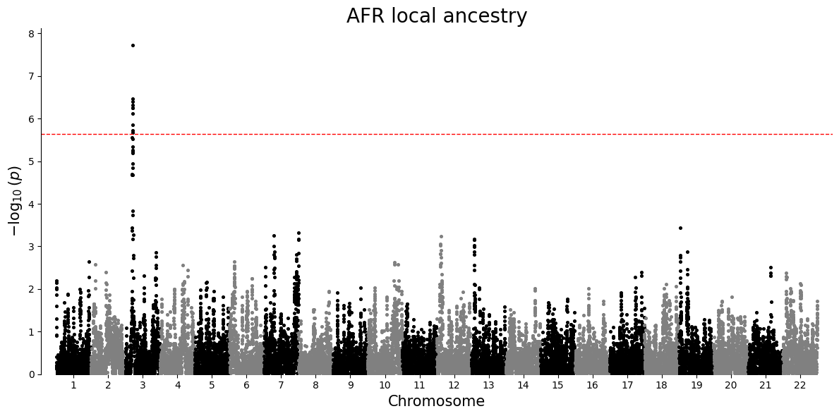
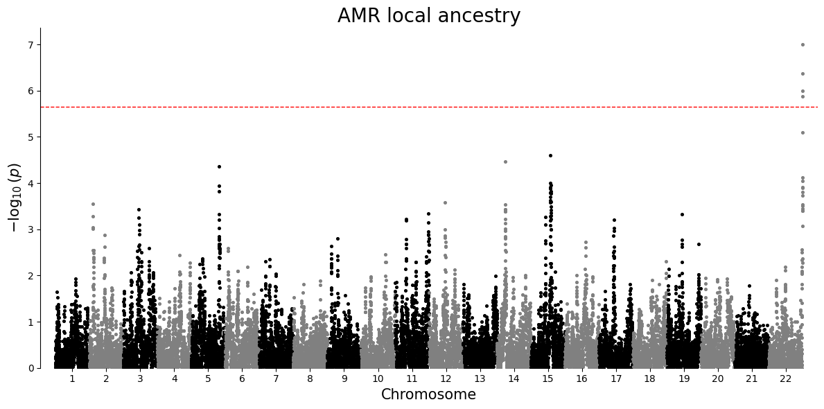
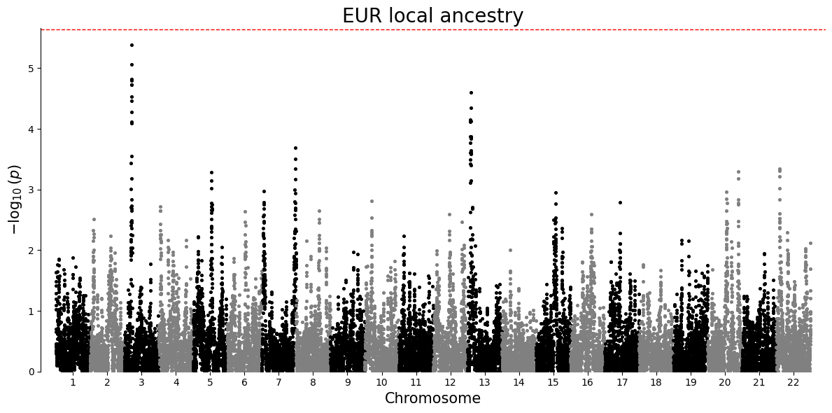
Manhattan plot

A Manhattan plot places association strength along genomic position. Each point is one local ancestry window for a single ancestry-specific test. Taller points have smaller p-values. The dashed line is a Bonferroni threshold, a strict correction that divides the chosen significance level by the number of tests in that ancestry-specific plot.

plot_df = results.loc[results["P"].notna() & (results["P"] > 0), ["#CHROM", "POS", "P", "ANCESTRY"]].copy()

for ancestry in sorted(plot_df["ANCESTRY"].unique()):
    ancestry_df = plot_df.loc[plot_df["ANCESTRY"] == ancestry, ["#CHROM", "POS", "P"]].copy()
    manhattan_plot(ancestry_df, title=f"{ancestry} local ancestry")

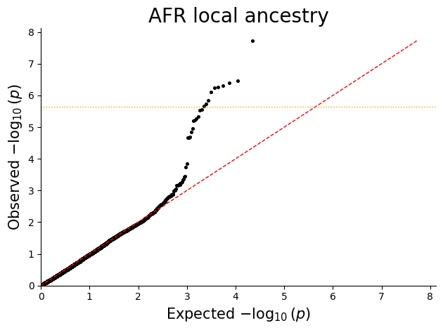
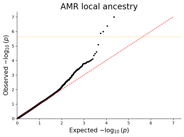
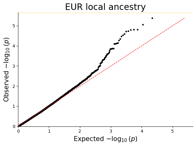
Q-Q plot

Q-Q plots help check whether the p-value distribution looks well calibrated under the null and highlight departures consistent with true signal or residual confounding.

for ancestry in sorted(plot_df["ANCESTRY"].unique()):
    ancestry_df = plot_df.loc[plot_df["ANCESTRY"] == ancestry, ["P"]].copy()
    qq_plot(ancestry_df, title=f"{ancestry} local ancestry")