Local Ancestry Visualization

Local ancestry can be viewed at two levels: chromosome paintings for individual genomes, and stacked cohort plots for many samples. This tutorial starts with full-chromosome paintings, then uses plot_lai for a dataset-level view.

Build full-genome local ancestry

build_synthetic_chromosome_painting_dataset() creates local ancestry windows across chromosomes.

from pathlib import Path

import matplotlib.pyplot as plt
import numpy as np
import pandas as pd
from IPython.display import Image, display

from snputils.datasets import build_synthetic_chromosome_painting_dataset
from snputils.visualization import chromosome_painting
from snputils.visualization.lai import plot_lai

RESULTS_DIR = Path("results/tutorials/local_ancestry")
RESULTS_DIR.mkdir(parents=True, exist_ok=True)
SEED = 20240520

painting_dataset = build_synthetic_chromosome_painting_dataset(
    n_samples=20,
    windows_per_chromosome=60,
    seed=SEED,
    build="hg38",
    ancestry_map={"0": "AFR", "1": "EUR", "2": "EAS"},
)

laiobj = painting_dataset["laiobj"]
build = painting_dataset["build"]
selected_samples = laiobj.samples[:3]

print(laiobj)
selected_samples

LocalAncestryObject(shape=(1380, 40), n_windows=1380, n_samples=20, n_haplotypes=40, n_ancestries=3, has_window_metadata=True, has_ancestry_map=True)

['sample0', 'sample1', 'sample2']

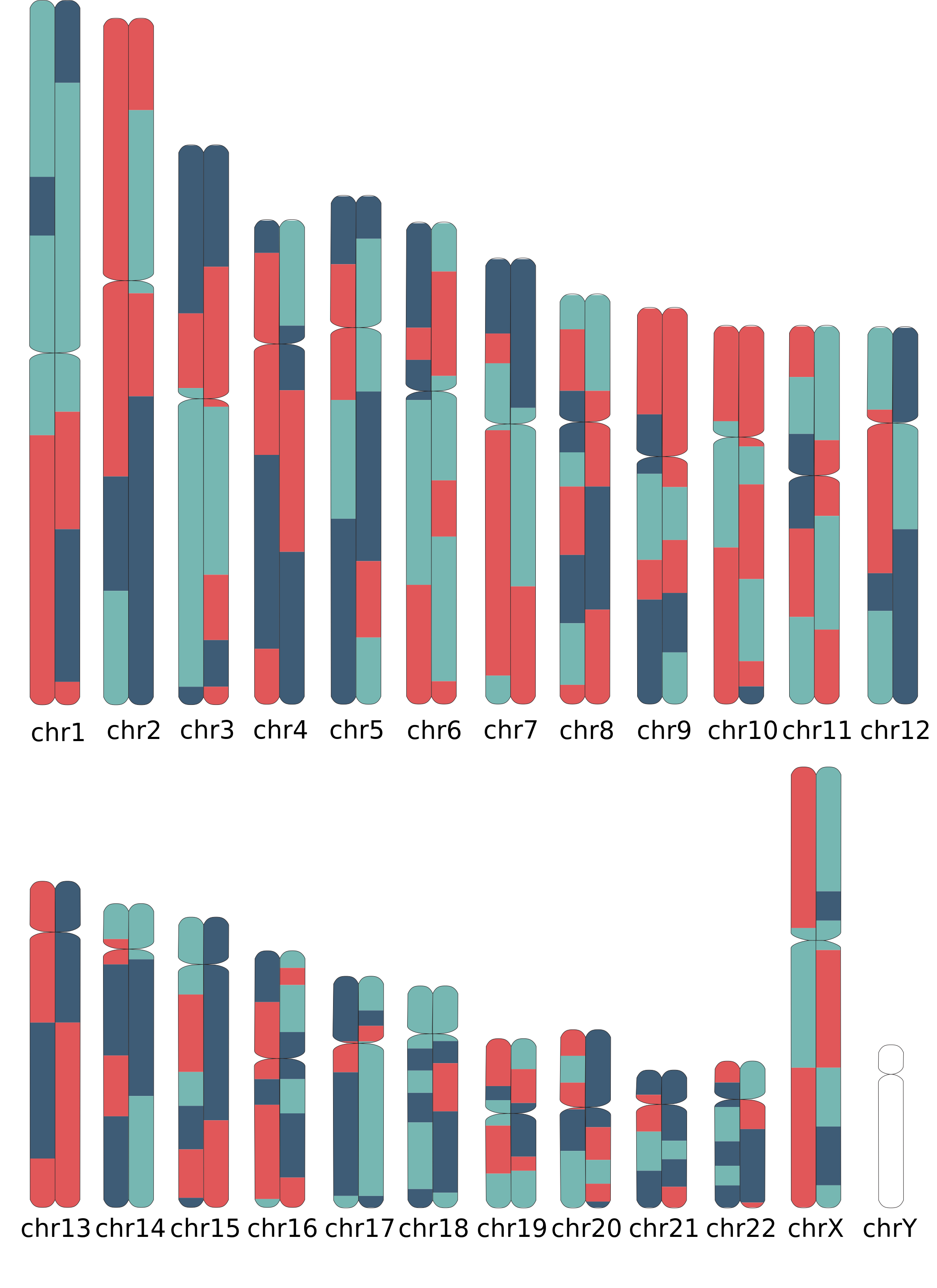
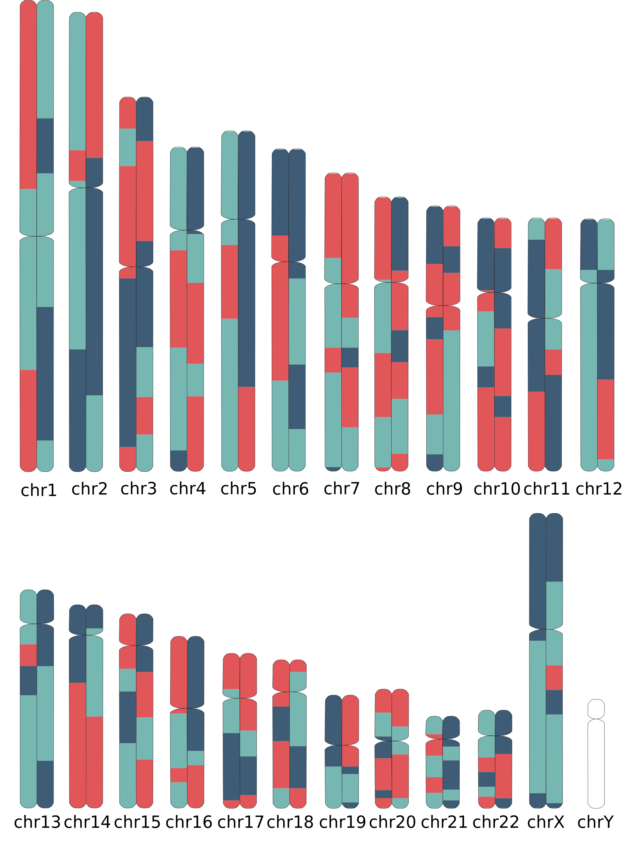
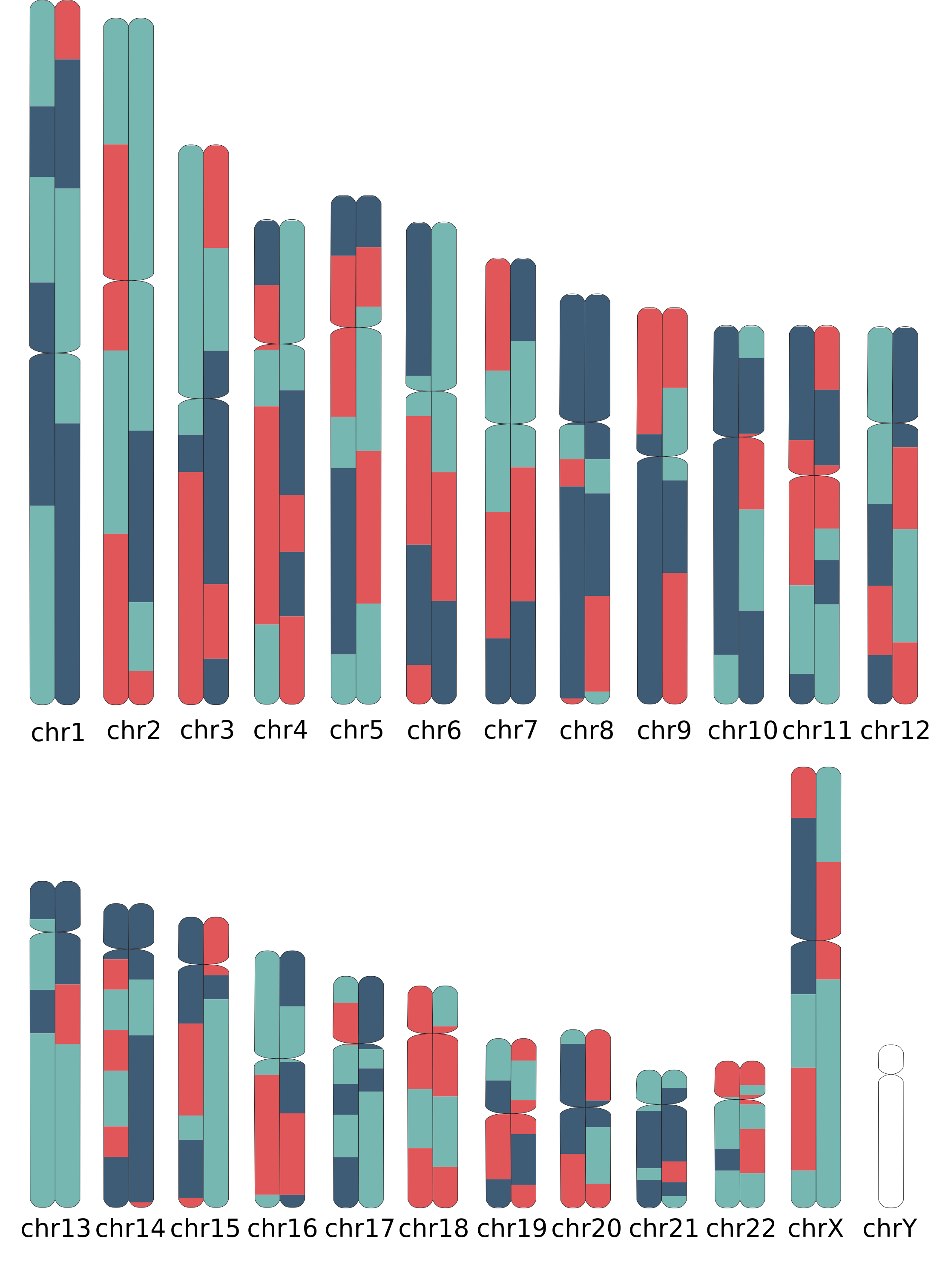
Paint full chromosome sets

chromosome_painting can use the LocalAncestryObject directly. Here we paint three selected samples and display the resulting PNGs.

from snputils.visualization.constants import get_palette_color

color_map = {0: get_palette_color(0), 1: get_palette_color(1), 2: get_palette_color(2)}

painting_outputs = chromosome_painting(
    source=laiobj,
    output_dir=RESULTS_DIR / "paintings_from_laiobj",
    sample_id=selected_samples,
    build=build,
    color_map=color_map,
    output_format="png",
    force=True,
    verbose=False,
    show=False,
)

for path in painting_outputs:
    display(Image(filename=path))

Chromosome painting 1/3 (sample0)
Chromosome painting 2/3 (sample1)
Chromosome painting 3/3 (sample2)

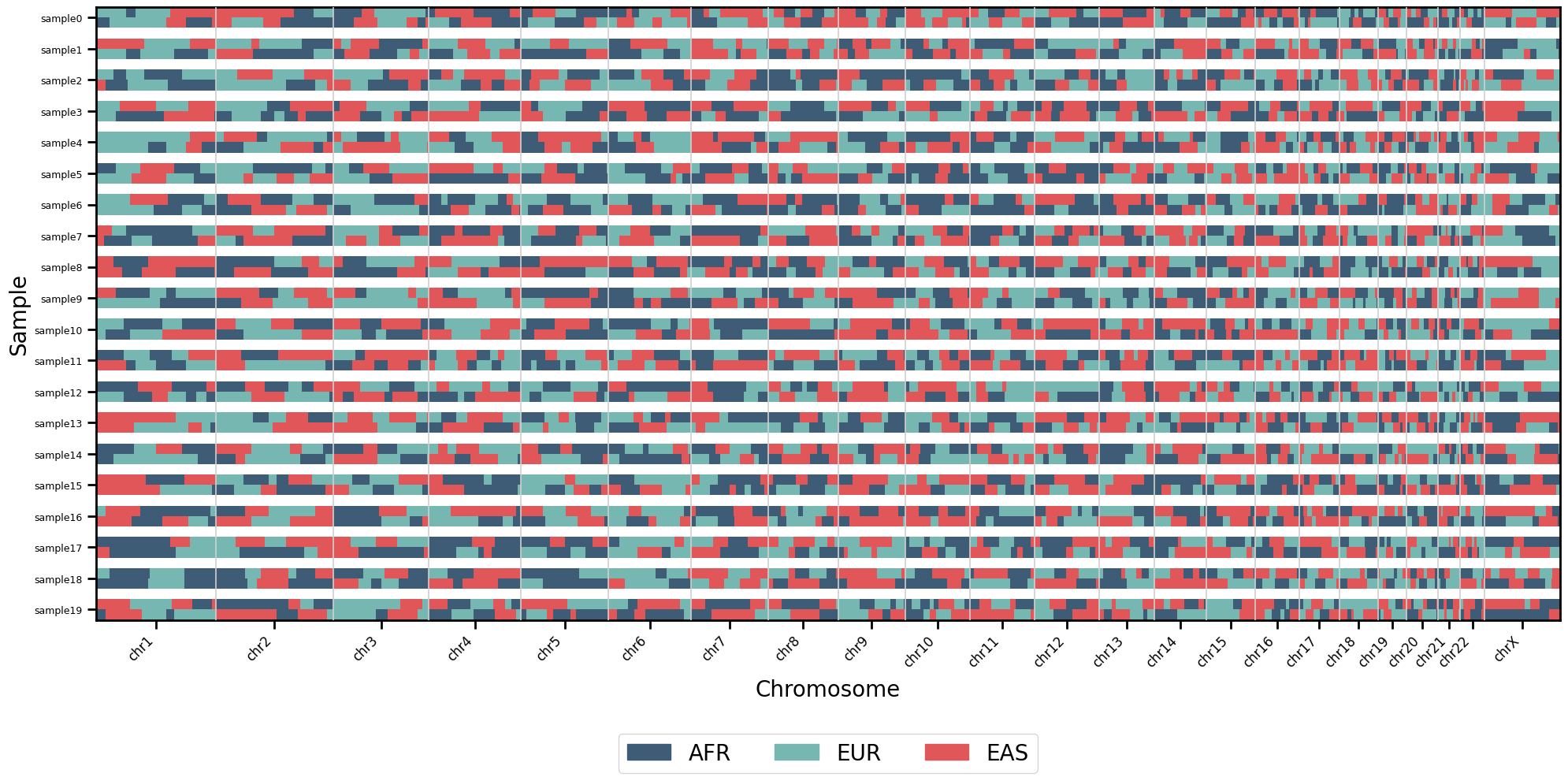
Dataset-level LAI plot

plot_lai shows many samples and windows in one matrix. For full-genome data, this is a compact overview rather than a chromosome-scale inspection tool; chromosome paintings above are better for reading one individual genome.

colors = {"AFR": get_palette_color(0), "EUR": get_palette_color(1), "EAS": get_palette_color(2)}

plot_lai(
    laiobj,
    colors=colors,
    sort=False,
    figsize=(20, 10),
    legend=True,
    scale=2,
)
plt.xticks(rotation=45, ha="right")
plt.tight_layout()
plt.show()

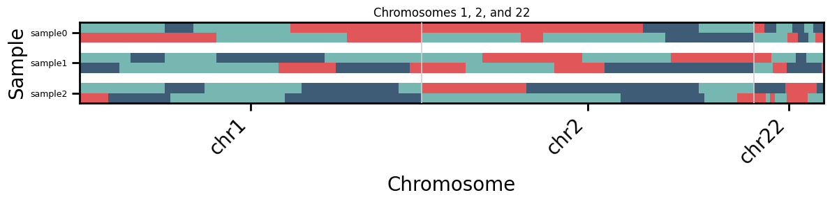
Focused cohort plot

For a closer matrix view, filter to a few chromosomes or samples. This example keeps the original sample order with sort=False.

focused_indexes = np.where(np.isin(laiobj.chromosomes.astype(str), ["1", "2", "22"]))[0]
focused = laiobj.filter_windows(indexes=focused_indexes)
focused = focused.filter_samples(samples=selected_samples, reorder=True)

plot_lai(
    focused,
    colors=colors,
    sort=False,
    figsize=(12, 3),
    title="Chromosomes 1, 2, and 22",
    scale=4,
)
plt.xticks(rotation=45, ha="right")
plt.tight_layout()
plt.show()